
When talking about flow data (netflow, sflow, jflow, IPFIX) statistics or summary of connections that transit through equipment such as switches, routers and firewalls immediately come to mind. In fact, these are the most common locations for capturing flow/traffic data and, probably, these locations will contain the greatest amount of relevant data, in addition to being where there is a greater possibility of obtaining more visibility regarding the network, however, capturing this information on servers it is also and can be useful for monitoring and visibility in some cases.
This type of strategy can be useful for network segments where there is no equipment with native capacity to export flow data, or to easily deliver a complete capture in the Packet Capture (PCAP) format, but it can also be used for monitoring home networks, as is the case of the small laboratory that will be shown in this article. This monitoring, among other advantages, can help you understand how data flows within the network, find problems (troubleshooting) and, of course, deliver a little more visibility to also help detect unusual, suspicious or malicious activities.
As mentioned in the previous article on Flow Data (here), 3 elements are needed to collect and analyze this data: an exporting equipment, a collector and an analyzer. In this hypothetical scenario, we will do everything on a single device, leaving the analysis software for a future article. The focus here is on how to get the data and analyze it a little more raw.
Information about the laboratory
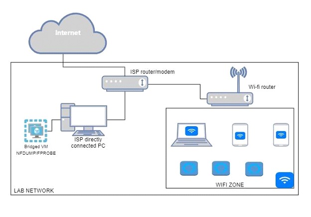
To carry out this export and collection work, two open source tools will be used: nfdump and fprobe, inside a virtual machine with Kali Linux installed. You need to configure the virtual machine to allow its network interface to enter promiscuous mode. In this scenario, the interface in promiscuous mode will allow you to see all the traffic, since it is a home network without segmentation: this includes traffic that is not destined for the VM or host interface, such as communications between other devices on the network.
It is possible that this lab will be reproduced in other Linux distributions and even in Windows machines, using similar concepts and tools. Below, a drawing of the structure of the home network where the tests will be carried out.
First, it's necessary to search for and install the utilities mentioned above, nfdump and fprobe. For organization purposes, configuring these softwares will be covered in two different sections of this article. Note: In the following examples, both softwares were installed using the package manager (apt – debian like) and no problems were found in operation, however note that the installation can be done manually using the source code from the developers.
Server configuration for stream data collection
NFDUMP will be responsible for capturing/collecting this data. According to the project's GitHub page, it's an open source software suite that allows collecting, processing and analyzing network stream data sent by compatible devices. Note that the nfdump suite will not be our flow data export software, but the collection one.

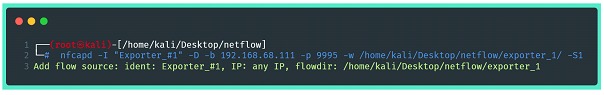
After installing nfdump, the utility will be available as nfcapd, which has the ability to function as a daemon, and will allow the opening of a socket to receive the stream data. To configure the utility to receive stream data, you need to run the command below:
Where:
⦁ -I “Exporter_#1”: define a string identification for the statistics file.
⦁ -D: throws the execution to the background
⦁ -p: define an UDP port in which the collector will listen
⦁ -w: defines the directory where the files will be stored flow
⦁ -S1: defines a storage scheme in subdirectories, in the following format: %Y/%m/%dd year/month/day (search in } man nfcapd(1) for more options, default is 0, no subdirectories).
The socket will open on the server, where stream data from any source can be pointed. Reminder: in this example, all elements will be present in only one server, and only one instance of the nfcapd. It is important to mention that this utility supports several instances of itself, making it possible to send data streams from different exporters (switches, routers, firewalls and why not servers?) and separate them by destination port on the server and by directories, for better data organization.
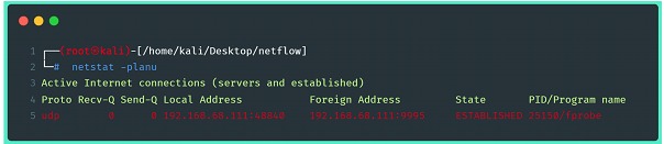
Using the command netstat -planu it is possible to identify the running service and its respective PID.
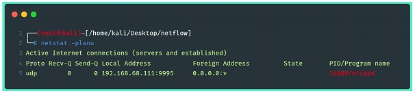
With these settings, the server is already able to receive stream edata at the address and port shown in the image. The next step is to configure it to capture and export the stream data.
Server configuration for exporting stream data
As previously mentioned, the software used to export the flow data will be fprobe, an open source tool, running on Linux-based systems for very lightweight network monitoring, used to collect and export real-time network flow data. In the absence of a more complete description in the manual/developer pages, the artificial intelligence model “ChatGPT” was asked to describe the characteristics of fprobe, and the text below was the result:
“fprobe works by listening for network traffic on a given interface and generating flow data based on the information collected. It can collect data over a variety of network protocols including TCP, UDP and ICMP. Data collected by fprobe includes information such as source and destination IP addresses, source and destination ports, and the amount of data transferred
One of fprobe's key features is its ability to export flow data to various flow collectors and analyzers, such as the popular network traffic analysis tool, ntopng. fprobe can export data in different formats including NetFlow and IPFIX.
Other fprobe features include:
⦁ Low CPU and memory usage, making it ideal for use on low-power devices
⦁ Support for multiple interfaces and IPv6 addresses
⦁ Configurable packet filtering options to capture specific types of traffic
⦁ ⦁The ability to generate reports in multiple formats, including ASCII and HTML”
Fprobe will be responsible for making the network interface enter promiscuous mode, listening to the traffic and exporting it to the pre-configured collector.To do so, you will need to follow a few steps, the first of which is to install the utility:

Once installed, the fprobe is now ready to be used. There are two ways to make it work: the first is to run the program as a command in shell, the problem with this is that it will always be necessary to run it manually, or include the command in some script initialization, scheduling or similar. The other way is to change the configuration file and make it run as a service. Both ways will fprobe run in the background, connected to a sink that is ready to receive the stream data.
Below, the command that will do the fprobe run instantly on shell:

Where:
⦁ -i eth0 – the interface that will be the target of the flow data export
⦁ dirección :port of the collection service
Note: fprobe, both in its “service” version and in its version run on the command line, has several operating and filtering options. The filters of fprobe are exactly the same as tcpdump and may be needed to select data, protocols, addresses, interfaces, ports, etc. In this example, we are using the simplest way of executing fprobe.
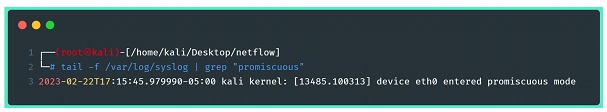
Once executed, it is possible to monitor the messages from the Linux kernel to identify if there was any error in the execution, or if the command was executed successfully:
Another possible check is to use the command netstat to view the connection between exporter and collector established:
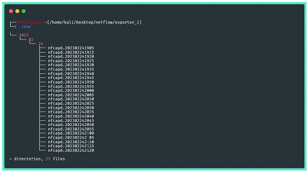
Once the connection between the collector and the exporter has been established, the flow data starts to be written in the directory previously indicated when configuring the collector.
Returning to the nfdump suite, to check the consistency of the stored stream data, we can use the analysis commands provided by the software. In the images below, there are some examples, but it is highly recommended that you consult the utility's help pages, as well as its manuals for applying filters and handling statistics. The first image shows a statistical summary of the captured data, containing information about everything sent by the exporter.
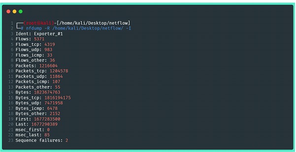
Where:
⦁ -R: reads the netflow content of a sequence of files and subdirectories of the indicated directory
⦁ -I: prints net flow statistics summary information for a file or range of files (-r or -R)
The next image brings information about the data transmitted in the extended format, provided by nfdump without any kind of filter. We can see information like timestamps, IP addresses, source and destination ports, number of packets, bytes, packets and bytes per second, and at the end, a summary:
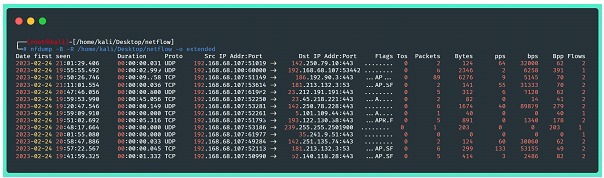
Where:
⦁ -B: adds the flows bidirectionally (considers round trip traffic)
⦁ -R: reads the netflow content of a sequence of files and subdirectories of the indicated directory
⦁ -o extended: indicates the output format (raw, line, long, extended, csv, json...))
Important note: if nothing is specified in the nfcapd configuration, the flow data will be “listened to” by the collector during cycles of 300 seconds, and only at the end of each cycle will new files be written to disk. Therefore, there is no reason to despair if the check described in the image above does not bring any results!
According to the need, as previously mentioned, it is possible to make fprobe run as a service by changing its configuration file. In a standard installation via apt (for debian like distributions) configuration file is located at /etc/default/fprobe, and its content is extremely intuitive:
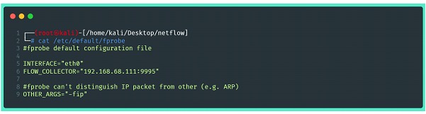
The options provided by the fprobe command, including filtering, must be included in the “OTHER_ARGS=” section. After correctly changing the configuration file, the next step is to activate the fprobe through systemctl and, if necessary, include it in the systemd for automatic startup.
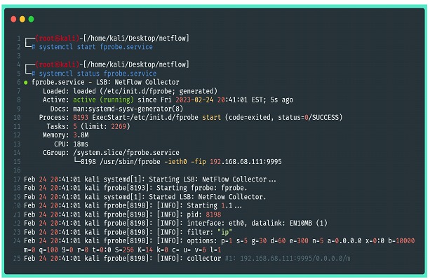
Once this is done, it is possible to return to the previous steps to verify if the service is correctly generating the files with the flow data.
Conclusions:
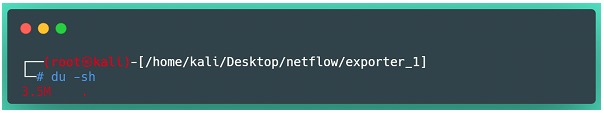
The purpose of developing content like this is to show that capturing flow data on servers is an extremely simple task to perform and that it can provide good information for monitoring operations. This type of collection does very well what it promises and effectively achieves the objective of delivering a little more visibility and understanding about the monitored network in the form of statistics at a very low cost: it is always important to remember that there is no raw data here, only metadata, which makes the operation very light and can help save disk space and processing.
To get an idea of the amount of data generated in terms of disk space, the lab environment was monitored for almost 72 uninterrupted hours and ended up occupying approximately 3.5 MB. Considering that it is a home network of small size, with just over 10 devices connected, but with a good flow of information, with long periods of video streams, online meetings and other connections, we were able to prove the savings in terms of data volume, especially when compared to other forms of traffic capture.
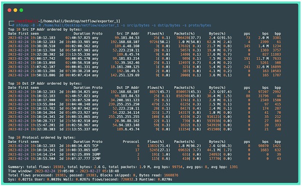
In this lab, it was possible to increase the visibility of a home network. The initial idea was to gain a better understanding of how the network works and be able to monitor the activities carried out by IoT devices such as smart switches and light bulbs that are connected to the internet. Below, as a last example, one more of the functions of the tool nfdump, which is to show the flow data statistics divided by “fields” present in the flows.
Where:
⦁ -B: adds the flows bidirectionally (considers round trip traffic)
⦁ -R: reads the netflow content of a sequence of files and subdirectories of the indicated directory
⦁ -s: it shows a Top 10 of the requested statistics, in the example above are highlighted source IPs sorted by bytes, destination IPs by bytes, and protocols by bytes. It should be noted that by default, the top 10 is shown, but this number can be changed by adding the option -n.
This scenario is perfectly portable to a larger environment and applicable in places where visibility, budget and monitoring capacity are limited. The next post, the last in this series, will address a more professional application of this type of monitoring, using an analysis tool with greater capacity for historical data visualization.

